An Investigation of the Agreement Among Hypothesis Tests for 2x2 Tables
This post is modified from a presentation I had given in April 2011 at the MAA Allegheny Mountain Section Meeting while in my Senior year of undergrad. My advisor was Dr. John Kern, a statistics professor at Duquesne University.
What is a 2x2 Table?
When collecting data for a study involving a binary response variable and a binary predictor variable, a 2x2 table can be used to display the results. Consider, for example, a study where a researcher is surveying a population on the prevalence of a disease against exposure to some kind of stimulus. The resulting 2x2 table would look like this:
| Exposed | Not Exposed | |
| Disease | a | b |
|---|---|---|
| No Disease | c | d |
Here, respondents in category a were exposed to the stimulus AND tested positive for the disease, respondents in category b were NOT exposed to the stimulus and did NOT test positive for the disease, etc. In the rest of this post, we will be exploring the following three questions of interest that can be answered using this data:
- Is the proportion of those with the disease among the exposed population significantly different from the proportion among the non-exposed population?
- Does someone's disease status depend on their exposure status?
- Are the odds of disease among those exposed different from the odds among those non-exposed?
In statistics, these are all common -- and related -- questions.
Exploring the Questions of Interest
Let's consider another example with a more specific premise. Consider the population of motorcycle accident victims. 79 are sampled, asking if they were wearing a helmet at the time of their accident and if they had sustained a facial injury. This results in the following 2x2 table:
| No Helmet | Helmet | |
| Facial Injury | 15 | 12 |
|---|---|---|
| No Facial Injury | 21 | 31 |
Revisiting question 1 above, we can rephrase it as, "Is the proportion of facial injury among non-helmet wearers significantly different from that among helmet wearers?" This can be answered with the z-test for difference in population proportions. There is evidence to answer "yes" if the following condition is met:
\( \lvert \frac{\frac{a}{a+c} - \frac{b}{b+d}}{\sqrt{\frac{a+b}{a+b+c+d} * \frac{c+d}{a+b+c+d} * \left( \frac{1}{a+c} + \frac{1}{b+d} \right) }} \rvert \)
For simplicity, we will refer to this equation as $$f_1(a,b,c,d)$$
Question 2 can be rephrased as, "Does facial injury depend on wearing a helmet?" This can be answered with the \( X^2 \) independence test, which uses this formula to calculate the test statistic:
\( \sum \frac{(O - E)^2}{E} \)
Where O is the observed value and E is the expected value. For a critical value with 95% probability with 1 degree of freedom, this allows us to answer "yes" if:
\( \frac{ \left( a - \frac{(a+b)(a+c)}{(a+b+c+d)} \right) ^2}{\frac{(a+b)(a+c)}{(a+b+c+d)}} + \frac{ \left( b - \frac{(a+b)(b+d)}{(a+b+c+d)} \right) ^2}{\frac{(a+b)(b+d)}{(a+b+c+d)}} + \frac{ \left( c - \frac{(a+c)(c+d)}{(a+b+c+d)} \right) ^2}{\frac{(a+c)(c+d)}{(a+b+c+d)}} + \frac{ \left( d - \frac{(b+d)(c+d)}{(a+b+c+d)} \right) ^2}{\frac{(b+c)(c+d)}{(a+b+c+d)}} \)
For simplicity, we will refer to this equation as $$f_2(a,b,c,d)$$
Finally, we can rephrase question 3 as, "Are the odds of facial injury among non-helmet wearers significantly different from that of helmet wearers?" We can answer this by using the confidence interval for a population odds ratio (ie the odds ratio test), which uses the following formula to create the confidence interval:
\( \exp \left( \ln(\frac{ad}{bc}) \pm 1.96 \sqrt{\frac{1}{a} + \frac{1}{b} + \frac{1}{c} + \frac{1}{d}} \right) \)
If this interval contains 1, then that would allow us to answer "Yes". However, we can simplify this further. If we apply the log to the interval and critical value, this would remove the exponential, as well as change the value to ln(1) = 0. We can then multiply the two interval formulas, as both formulas resulting in the same sign means that 0 cannot be included in the interval. Thus, we can say that it will allow us to answer "Yes" if:
\( \left( \ln(\frac{ad}{bc}) - 1.96 \sqrt{\frac{1}{a} + \frac{1}{b} + \frac{1}{c} + \frac{1}{d}} \right) * \left( \ln(\frac{ad}{bc}) + 1.96 \sqrt{\frac{1}{a} + \frac{1}{b} + \frac{1}{c} + \frac{1}{d}} \right) > 0 \)
For simplicity, we will refer to this equation as $$f_3(a,b,c,d)$$
If we enter the numbers in our 2x2 table into these formulas, the tests produce the following results:
- z-test: \( f_1(15,12,21,31) = 1.28 < 1.96 \)
- Not enough evidence to answer "yes"
- \( X^2 \) test: \( f_2(15,12,21,31) = 1.65 < 3.841 \)
- Not enough evidence to answer "yes"
- Odds ratio test: \( f_3(15,12,21,31) = -0.512 < 0 \)
- Not enough evidence to answer "yes"
Thus, all three tests are in agreement.
Example Revisited
What if we observed something slightly different?
| No Helmet | Helmet | |
| Facial Injury | 15 | 8 |
|---|---|---|
| No Facial Injury | 21 | 31 |
If we apply the same tests with this changed value, we get the following results:
- z-test: \( f_1(15,8,21,31) = 1.98 > 1.96 \)
- Enough evidence to answer "yes"
- \( X^2 \) test: \( f_2(15,8,21,31) = 3.94 > 3.841 \)
- Enough evidence to answer "yes"
- Odds ratio test: \( f_3(15,8,21,31) = -0.668 < 0 \)
- Not enough evidence to answer "yes"
In this example, there is a disagreement between the odds ratio test and the other two tests.
Note that it is known that the z-test and \( X^2 \) test always produce the same result. This can be proven using the "simplify" function in Matlab to show that \( f_1^2 = f_2 \). Because of this, we will use the \( X^2 \) test and no longer need to observe the z-test. To explore the discrepancies between the \( X^2 \) test and the odds ratio test, we have created a simulation.
Simulation
The following population was chosen randomly:
| \( E \) | \( \bar{E} \) | |
|---|---|---|
| \( D \) | 75 | 75 |
| \( \bar{D} \) | 30 | 30 |
A sample of size 75 was taken from this population, with replacement. Then, \( f_2 \) and \( f_3 \) were calculated and compared to their respective test values (3.841 and 0). The results of the test were noted and recorded in a separate 2x2 table.
For example, say that the following sample is taken from this population:
| \( E \) | \( \bar{E} \) | |
|---|---|---|
| \( D \) | \( a = 21 \) | \( b = 29 \) |
| \( \bar{D} \) | \( c = 10 \) | \( d = 15 \) |
We then apply the two tests and find the following results:
- \( X^2 \) test: \( f_2(21,29,10,15) = 0.02 < 3.841 \)
- Not enough evidence to answer "yes"
- Odds ratio test: \( f_3(21,29,10,15) = -0.948 < 0 \)
- Not enough evidence to answer "yes"
Since both tests answer "no", we can increment that value in an agreement table:
| OR = Yes | OR = No | |
|---|---|---|
| \( X^2 \) = Yes | \( 0 \) | \( 0 \) |
| \( X^2 \) = No | \( 0 \) | \( 1 \) |
This process was performed for 10,000 simulations, resulting in the following agreement table:
| OR = Yes | OR = No | |
|---|---|---|
| \( X^2 \) = Yes | \( 500 \) | \( 44 \) |
| \( X^2 \) = No | \( 0 \) | \( 9456 \) |
We can see from this table that most iterations ended in agreement between the tests. However, there were a small number of iterations that showed disagreement. In these disagreements, the odds ratio test would return "no", while the \( X^2 \) test would return "yes" (44 simulations). It was never the case where the odds ratio test would return "yes", while the \( X^2 \) test would return "no". That is, simulations suggest that if \( f_2 < 3.841 \) (\( X^2 \)test "no"), then the same (a,b,c,d) CANNOT yield \( f_3 > 0 \) (odds ratio "yes"). To get more insight into these disagreements, we created a computational proof.
Written in Java, the brute force proof checks every possible (a,b,c,d) combination of integers of the interval [1,1000]. All disagreements were recorded. If \( f_2 < 3.841 \), then the program checks if \( f_3 < 0 \). As expected, no such cases of this disagreement were found. Thus, a \( X^2 \) test "no" and odds ratio test "yes" is impossible to observe for (a,b,c,d) up to and including 1000. QED
In all, the interval [1,1000] among 4 variables results in 1 trillion combinations. In these combinations, there were 189,678,390 disagreements, or 0.019%. Curiously, there were FAR more disagreements at lower values of (a,b,c,d) than higher values. For example, at the following values of a:
- a=1: 4,582,424 disagreements among 1,000,000,000 combinations (0.458%)
- a=1000: 120,995 disagreements among 1,000,000,000 combinations (0.012%)
Additionally, patterns emerged in the disagreement data. The following shows an ordered run of disagreements:
| a | b | c | d |
|---|---|---|---|
| 1 | 84 | 86 | 998 |
| 1 | 84 | 86 | 999 |
| 1 | 84 | 86 | 1000 |
| 1 | 85 | 1 | 5 |
| 1 | 85 | 1 | 6 |
| 1 | 85 | 1 | 7 |
| 1 | 85 | 1 | 822 |
| 1 | 85 | 1 | 823 |
| 1 | 85 | 1 | 824 |
We can see that disagreements tended to "clump" around certain ranges of values.
Regrettably, the Java code and results are either lost to time, or are buried on an old computer's hard drive somewhere. Given that this simulation was created in 2011, recovery is quite unlikely.
Number of Disagreements vs. Sample Size
To see if our discovery of high disagreement with lower (a,b,c,d) was consistent, we repeated the simulation among multiple populations with different sample sizes n, arbitrarily chosen at {50, 75, 100, 250, 500, 1000, 2500, 5000}.
The first population we chose was the same as in the original simulation:
| 75 | 75 |
|---|---|
| 30 | 30 |
We ran the simulation multiple times with each of the sample sizes, then counted the number of disagreements that were found in each. We then averaged these counts for each sample size. As an example, typical agreement tables at n = 75 and n = 5000 looked like this:
| n=75 | OR = Yes | OR = No |
|---|---|---|
| \( X^2 \) = Yes | \( 476 \) | \( 48 \) |
| \( X^2 \) = No | \( 0 \) | \( 9476 \) |
| n=5000 | OR = Yes | OR = No |
|---|---|---|
| \( X^2 \) = Yes | \( 472 \) | \( 0 \) |
| \( X^2 \) = No | \( 0 \) | \( 9528 \) |
This highlights the difference in disagreements between small sample sizes and large sample sizes. Further emphasizing this is the resulting plot for the number of disagreements vs. sample size:
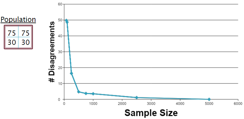
As expected, when the sample size increases, the number of disagreements decreases.
We were curious how different populations would affect the number of disagreements, though. For the second simulation, we created a population where all quadrants were of equivalent size:
| 10 | 10 |
|---|---|
| 10 | 10 |
Again, we ran the simulation multiple times with the same sample sizes, resulting in agreement tables looking like these:
| n=50 | OR = Yes | OR = No |
|---|---|---|
| \( X^2 \) = Yes | \( 434 \) | \( 128 \) |
| \( X^2 \) = No | \( 0 \) | \( 9438 \) |
| n=5000 | OR = Yes | OR = No |
|---|---|---|
| \( X^2 \) = Yes | \( 469 \) | \( 0 \) |
| \( X^2 \) = No | \( 0 \) | \( 9531 \) |
We see a larger number of disagreements for the small sample sizes, but the large sample sizes are nearly identical.
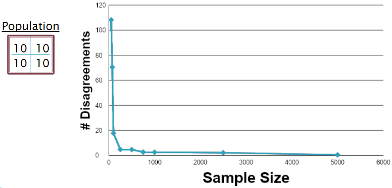
The plot agrees with that assessment: disagreements ARE much higher at small samples, but they still converge to 0 at large samples. Interestingly, even with the initial higher number of disagreements, it drops off MUCH more quickly than in the first population.
For the final population, we created a population where the top left and bottom right quadrants were equal, as were the top right and bottom left quadrants:
| 10 | 15 |
|---|---|
| 15 | 10 |
After running the simulations for the various sample sizes, we found some interesting results:
| n=50 | OR = Yes | OR = No |
|---|---|---|
| \( X^2 \) = Yes | \( 2717 \) | \( 335 \) |
| \( X^2 \) = No | \( 0 \) | \( 6948 \) |
| n=5000 | OR = Yes | OR = No |
|---|---|---|
| \( X^2 \) = Yes | \( 10000 \) | \( 0 \) |
| \( X^2 \) = No | \( 0 \) | \( 0 \) |
For small samples, we found a MUCH higher number of disagreements, as well as far more Yes-Yes agreements than the other populations. Additionally, we reach full Yes-Yes agreement at a relatively small number of samples, so we had to cut the simulation off there.
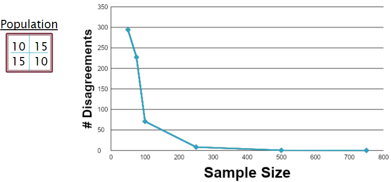
Disagreements ARE, in fact, much higher earlier on, and the also fall off much faster, already approaching 0 around 500 samples.
Conclusions
At the time, our research on such disagreements and disagreement patterns was ongoing, but it has since been abandoned due to my graduating from undergrad. If we were to revisit it today, we would likely investigate values higher than 1000 in the simulation data, as my computer was unable to run more combinations in a reasonable timeframe. Given the rise of solid state drives, higher capacity storage, and general processor improvements, we would likely be able to run FAR more simulations in the same amount of time.
Going back to the tests behind the disagreements, in what situations would you use one method over the other? According to Bret Larget, then at the University of Wisconsin, one such reason is audience familiarity.
If one of the tests is directly related to an estimate that is important in the field, this is also helpful. In medical statistics, risks are commonly described with odds ratios and so a test based on them can be more informative than just a p-value.-Bret Larget, 2011
In a more ethically questionable scenario, consider someone who is feeling the pressure to publish their study. Typically, studies that come to a solid conclusion (a "yes", in this case) tend to be published more often than those that fail to reject the null hypothesis (a "no"). Thus, if their results are borderline, they may want to use the test more likely to give that "yes".
References
[1] Peck, Roxy, Chris Olsen, and Jay Devore. Introduction to Statistics and Data Analysis. 3rd. Belmont, CA: Thomson Brooks/Cole, 2008. 620-25.
[2] Triola, Marc, and Mario Triola. Biostatistics for the Biological and Health Sciences. 1st. Boston: Pearson, 2006. 505-10.
[3] Pagano, Marcello, and Kimberlee Gauvreau. Principles of Biostatistics. 2nd. Pacific Grove, CA: Duxbury, 2000. 352-57.